The MOD function in Microsoft Excel lets you work out whether one number is divisible by another. If it’s not, it tells you what’s left over. For example, if you divide 3 by 2, the MOD function will return 1. In this guide, I’ll show you how you can use it to solve real-world problems.
The MOD Function Syntax
Before I show you the MOD function in action, let’s take a moment to see how it works:
=MOD(n,d)
where n is the number you want to divide, and d is the divisor. So, if you want to divide 3 by 2, 3 is the number, and 2 is the divisor.
If the divisor is negative, the result will also be negative. On the other hand, if the divisor is 0, Excel will return the #DIV/0! error, since you can’t divide a number by zero.
However, the MOD function is rarely used on its own—its true value really comes to the fore when it’s used alongside other Excel functions and tools.
Example 1: Using the MOD Function to Minimize Leftovers
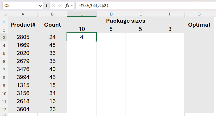
Let’s say you have various items that you want to package and distribute. Column A contains the product ID, column B tells you how many of each product you have, and row 2 contains the different package sizes. Your aim is to work out the optimal package size for each product, depending on how many of each product you have.
In this case, you can use the MOD function to tell you whether the product count in column B is divisible by the package size in row 2, and if it isn’t, how many you have left over.
So, in cell C3, type:
=MOD($B3,C$2)
The dollar symbol ($) placed before a row or column reference—also known as a mixed reference—tells Excel to lock it so that the formula can be applied to other cells in the range.
When you press Enter (or Ctrl+Enter to stay in the same cell), you can see that if you use a package with 10 spaces for product 2805, four will remain unpacked.
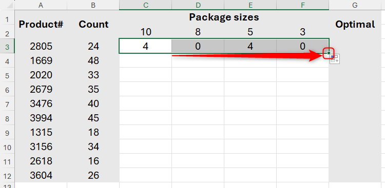
Now, when you click and drag the fill handle in cell C3 to the right to complete the row, you can see that using packages with eight or three spaces is ideal for this product.
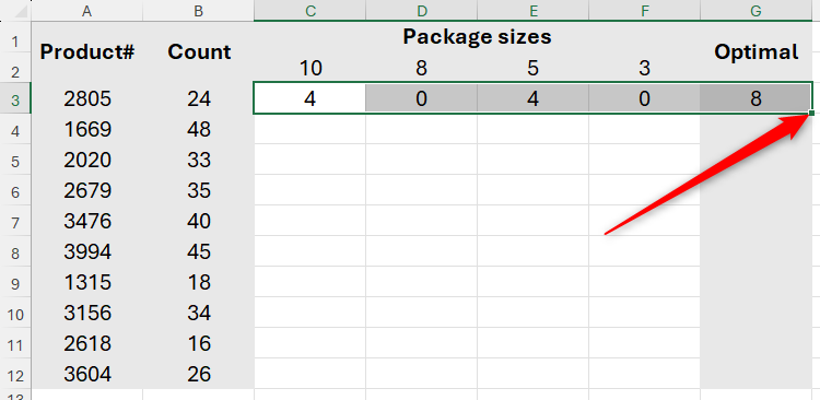
Next, in cell G3, you want Excel to tell you the best package size to use for that product. To do this, use INDEX and XMATCH:
=INDEX($C$2:$F$2,1,XMATCH(SMALL(C3:F3,1),C3:F3))
where INDEX($C$2:$F$2,1 tells Excel to return a value from cells C2 to F2, and XMATCH(SMALL(C3:F3,1),C3:F3)) looks up the smallest value in cells C3 to F3 to define the column number that feeds the INDEX part of the formula.
Finally, select cells C3 to G3, and double-click the fill handle to duplicate all the formulas to the remaining rows in the range.
Now, thanks to the MOD function being used in cells C3 to F12, column G tells you the best package sizes to use for each product, and you can look in columns C to F for each product to see how many (if any) you will have left over after using this optimal package size.
If the smallest value occurs twice in a row, XMATCH uses the first instance from left to right by default. In this case, this is ideal because you want to use as little packaging as possible.
The beauty of using this combination of functions is that if the product count in column B changes, the optimal package size updates according to the MOD formulas you used in cells C3 to F12. For example, if you originally miscounted product 2805, and you actually have 25 instead of 24, when you update the value in cell B3, you find that the optimal package size changes to five.
Example 2: Using the MOD Function to Highlight Certain Cells
Excel’s MOD function doesn’t have to be used to return a value—it can also be used to determine which cells should be formatted through conditional formatting.
In this example, imagine you want to create activities for ten groups of people. However, different activities require different numbers of subgroups, so you need to determine which groups can carry out which activity, ensuring all members are involved.
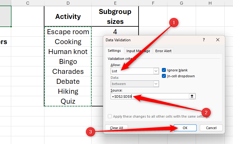
First, in cell B1, you want to create a drop-down list of the activities in column D. To do this, with cell B1 selected, head to the “Data” tab on the ribbon, and click the top half of the “Data Validation” button.
Second, in the Allow field of the Data Validation dialog box, choose “List.” Next, place your cursor in the Source field, and select the cells containing the values you want to appear in the drop-down list. Then, click “OK.”

Related
How to Add a Drop-Down List to a Cell in Excel
It beats typing in the same options 200 different times manually.
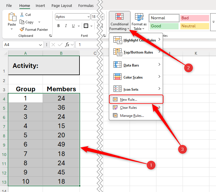
Now, when you select cell B1, you can see a drop-down list of activities, and you’re ready to apply formatting to cells A4 to B13 that tells you whether each group can carry out each activity.
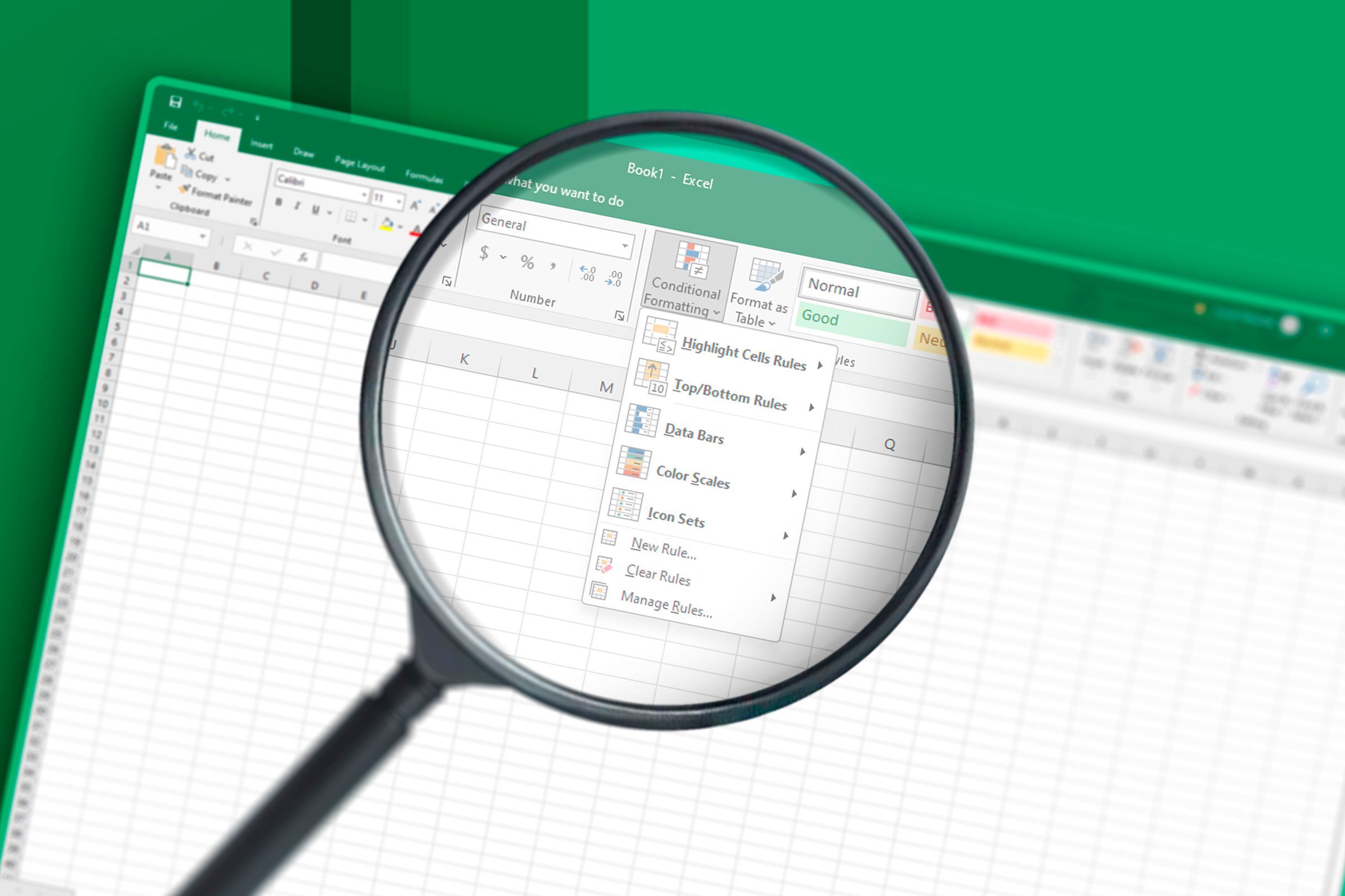
To do this, select cells A4 to B13, and in the Home tab on the ribbon, click Conditional Formatting > New Rule.
Related
I Use Conditional Formatting in Most Spreadsheets: Here’s Why
Conditional formatting is a non-negotiable.
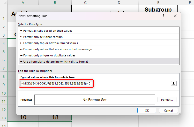
Then, in the New Formatting Rule dialog box, select “Use A Formula To Determine Which Cells To Format,” and in the formula field, type:
=MOD($B4,XLOOKUP($B$1,$D$2:$D$9,$E$2:$E$9))=0
where
- $B4 is the first of the cells in column B acting as the number to be divided,
- XLOOKUP($B$1,$D$2:$D$9,$E$2:$E$9) looks up the value in cell B1 and returns the corresponding subgroup size from the lookup table (the divisor), and
- =0 applies formatting to cells where the number of members in a group is divisible by the number of people required in an activity’s subgroup.
Placing the dollar symbol before the column reference ($B4) in this formula tells Excel that you want the formatting to be conditional on all selected cells in column B.
In other words, you want Excel to format the groups where the whole group size is divisible by the subgroup size required for the activity selected in cell B1.
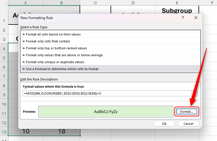
Finally, click “Format” to choose the formatting for the cells where these conditions are met. In my case, I’ve gone for a light green cell background.
Click “OK” to close the dialog box.
Now, select an activity in the drop-down menu in cell B1, and the groups that can participate in that activity will be highlighted according to the formatting you selected. In this example, you can see that groups 1, 2, 3, 5, and 8 can take part in the quiz because the total number of members in those groups is divisible by the subgroup size required for this activity.
On the other hand, when you select “Hiking” from the list, only group 5 is identified as being able to do this activity, as it’s the only group whose overall number is divisible by the subgroup size.
Example 3: Using the MOD Function to Spit Date-Time Values
Microsoft Excel’s MOD function can be used to extract the decimal part of a number. In this example, typing:
=MOD(A2,1)
into cell B2 divides 10.2 by 1, and tells you that the remainder of this division is 0.2.
You can also extract the integer from this number using the INT function, which rounds a value down to the nearest whole number. So, typing:
=INT(A2)
into cell C2 removes the decimal from the value in cell A2, returning the whole number only.
In the same way, you can use MOD and INT to split date-time values.
Here, cell A2 contains a date and time, and cell A3 contains the corresponding serial number.
Excel stores dates and times as serial numbers, which can be seen when you change the number format to “General.” So, in this example, the values of cells A2 and A3 are identical, but the number format for cell A2 is a custom date-time number format, while the number format for cell A3 is the general number format.
In the serial number in cell A3, 45782 represents the date, and 0.4375 represents the time, and you can use MOD and INT to split these up.
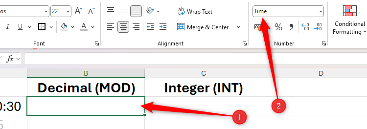
First, select cell B2, and change the number format to “Time” in the Number group of the Home tab on the ribbon.

Related
Excel’s 12 Number Format Options and How They Affect Your Data
Adjust your cells’ number formats to match their data type.
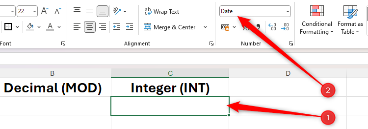
Then, select cell C2, and change the number format to “Short Date.”
Then, go back to cell B2, and type:
=MOD(A2,1)
This extracts the decimal (time) from the serial number representation of the date-time value in cell A2, and because you set the cell number format to Time, it converts the serial decimal to a time value.
Finally, go back to cell C2, and type:
=INT(A2)
This extracts the integer (date) from the serial number in cell A2 by rounding it down to the nearest whole number, and since you set this as a short date number format, it converts the serial integer to a date value.
Half the battle with using functions in Microsoft Excel is knowing which one is best for solving your problem. For example, if you want to refine your calculations, the AGGREGATE function will probably do the trick, and if you want to create a list of numbers, the SEQUENCE function is your best bet. Luckily, Excel is here to help you find the function you need—you can click the “fx” button next to the formula bar or search for a function in the Insert Function dialog box, and Excel’s function tools will help you along the way as you craft the perfect formula.

