Paste Special is an underrated tool in Microsoft Excel, with many people only using it to paste values. But it can do much more than that! Whether this is the first time you’ve heard of Paste Special or you’re a seasoned Excel pro, these tips and tricks are guaranteed to save you lots of time.
The keyboard shortcut for Paste Special in Microsoft Excel 365 (the version used in this article) and Microsoft Excel 2024 onward is Ctrl+Alt+V. However, in older versions, the keyboard shortcut is Ctrl+Shift+V.
1
Increase or Decrease Many Values by the Same Amount
You can use Paste Special to make wholesale changes to values in your Microsoft Excel spreadsheet.
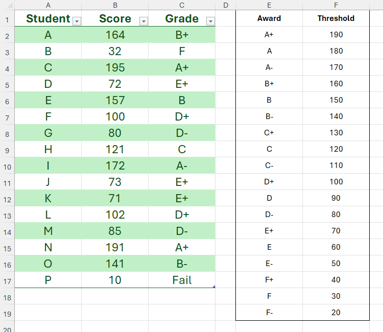
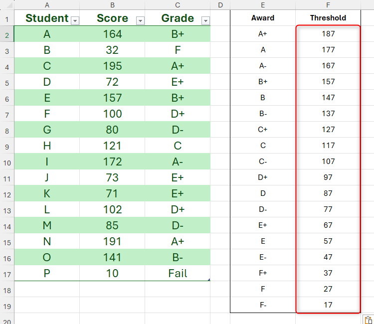
In this example, let’s say you’ve used XLOOKUP to return student grades based on the thresholds in the lookup table.
However, you later realize that the grade boundaries are too stringent, so you want to reduce all the thresholds by three points.
Instead of doing this manually, you could do a simple sum in another column, before replacing the old thresholds with the new ones. However, this method will take too long, especially when you can use Paste Special to do the same thing in fewer steps.
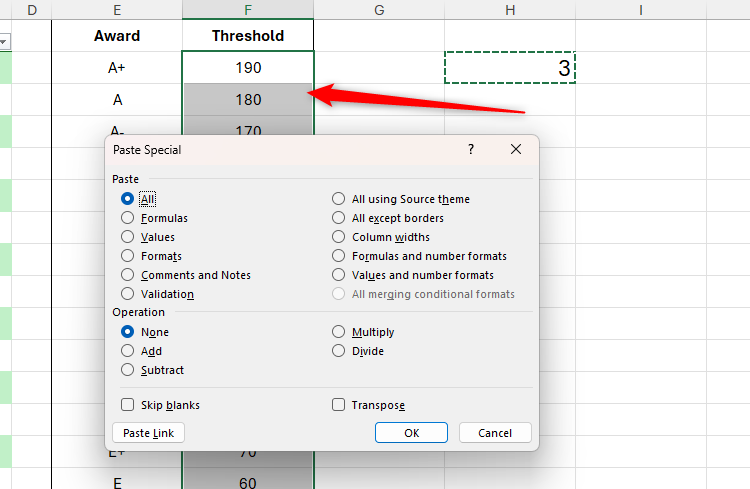
First, in a blank cell, type 3, as this is the decrease you want to apply to all the thresholds. Then, press Ctrl+C to copy that cell.
Next, with the influencer cell still copied, select all the cells containing the values you want to increase or decrease, and press Ctrl+Alt+V to launch the Paste Special dialog box.
The dialog box differs depending on what you’ve copied and selected. For example, when duplicating a chart’s formatting to another chart, you only have three options: paste all, paste formats, and paste formulas.
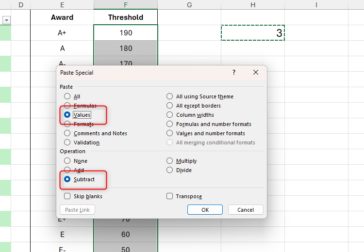
Now, press the keys that correspond to the underlined characters in the actions you want to perform. In this case, you want to perform the subtraction operation, so press S, and you only want to copy the value (not the formatting), so press V.
Finally, when you press Enter, you’ll see all the thresholds decrease by 3, and the cells have retained their original formatting, including the border and smaller font size.
Remember to clear the influencer cell once you’re done!
2
Turn Whole Numbers Into Percentages
If you’ve ever tried changing a whole number to a percentage, you’ll know all too well that Excel doesn’t make it easy to do.
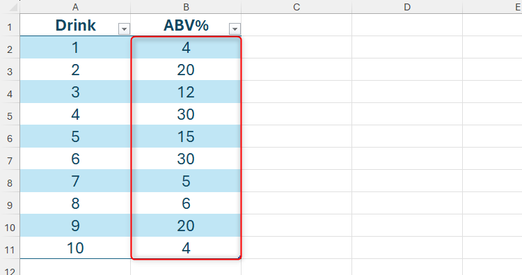
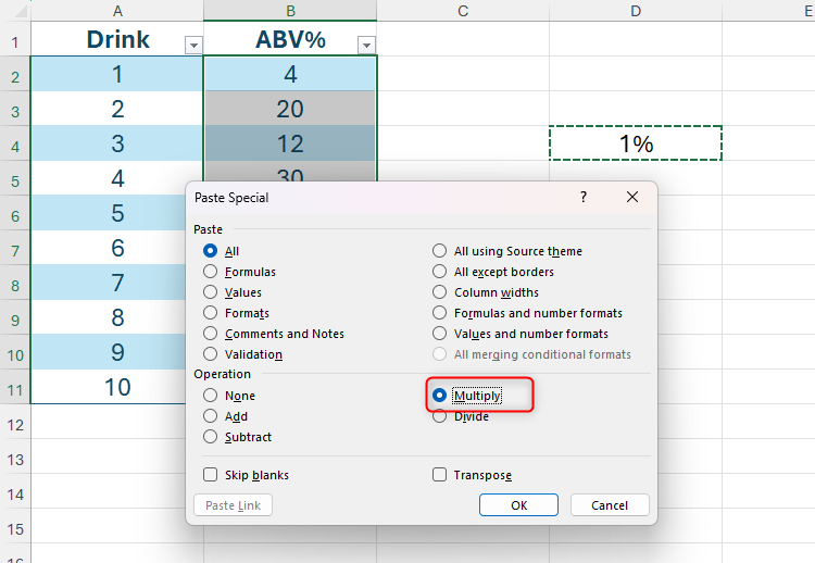
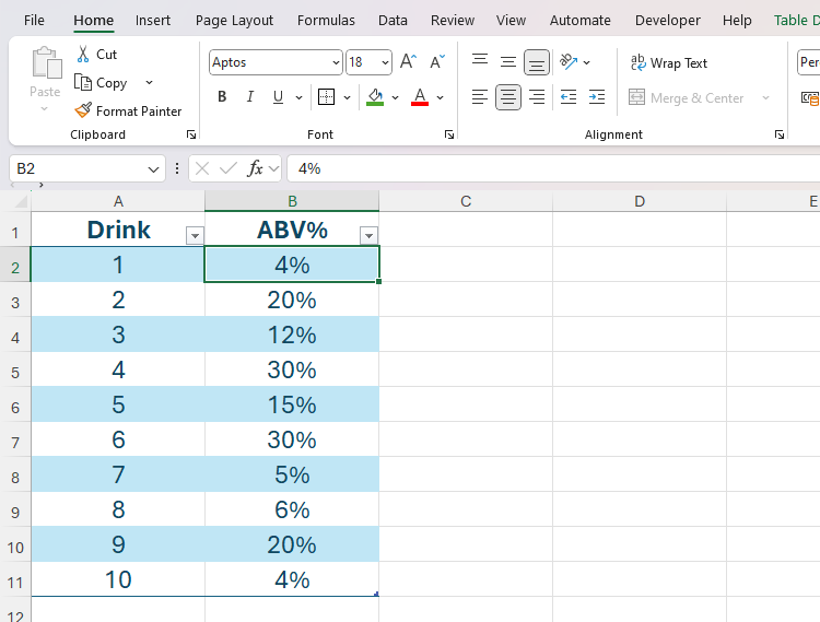
For example, imagine you’ve been sent this spreadsheet, and you want to turn the values in column B into percentages.

Related
Excel’s 12 Number Format Options and How They Affect Your Data
Adjust your cells’ number formats to match their data type.
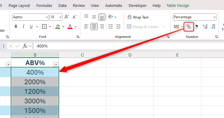
However, if you select the relevant cells and click the “Percentage” symbol in the Number group of the Home tab on the ribbon, since the values are whole numbers, they’ll convert to larger percentage values than you were hoping for.
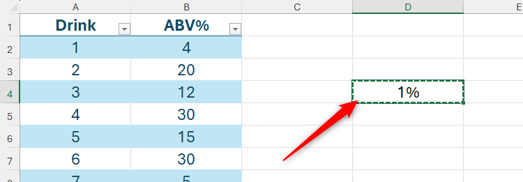
Instead, with the whole numbers in their original format, type 1% into a blank cell, and press Ctrl+C to copy it.
Now, select the cells containing the values you want to convert from whole numbers into percentages, and press Ctrl+Alt+V. Then, press M to activate the multiplication operation.
If the influencer cell is formatted differently from the cells you want to affect, remember to also press V to copy the values only.
Finally, press Enter, and all the whole numbers will be converted to their intended percentages. You can also clear the influencer cell, since it’s not linked in any way to the values in column B.
With Paste Special in Microsoft Excel, you can copy and paste more than a cell’s contents or formatting. Indeed, you can also duplicate a cell’s comment or note in another cell.

Related
Comments vs. Notes in Microsoft Excel: What’s the Difference?
Don’t get overwhelmed by annotations in Excel.
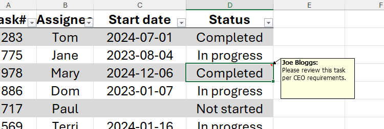
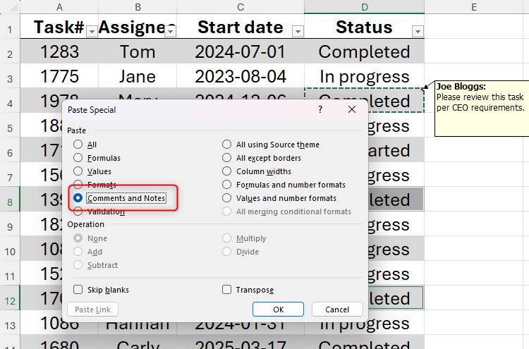
In this spreadsheet, let’s say you’ve added a note to a cell to indicate that a task needs further attention.
You then realize that other tasks also need to have the same note attached to them. Yes, you could copy the text in the note and duplicate it manually, but using Paste Special is a much quicker route. You could also use Ctrl+C and Ctrl+V to copy the whole cell, including its comments and notes, but this method causes issues if the cells are formatted differently.
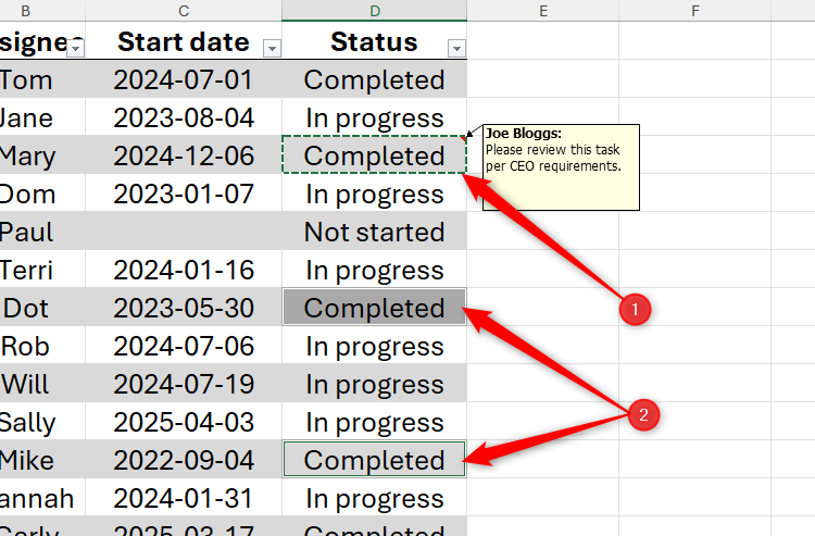
First, select and copy the cell containing the note, and then select the cell or cells where you want the note to be duplicated.
Press Ctrl while selecting non-adjacent cells to select them together.
Now, press C to select “Comments And Notes.”
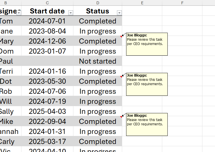
Finally, press Enter to see the note duplicated to the selected cells.
If you use the same method to copy comments between cells, the timestamp in the duplicated comment or comments will be the same as the timestamp in the original comment. In other words, the timestamp doesn’t update to indicate when the comment was duplicated through Paste Special.
4
Switch Rows and Columns
It’s fair to say that all the Paste Special tools are designed to speed up your workflow in Microsoft Excel. However, the most powerful of all the Paste Special options lets you switch rows and columns in your data.
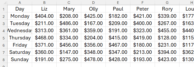
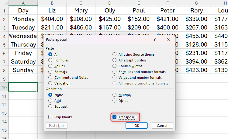
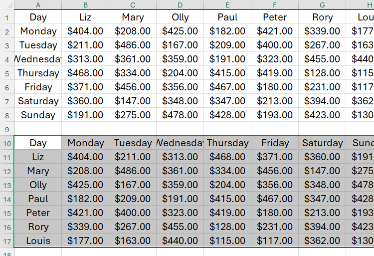
In this example, let’s imagine you’ve received this spreadsheet, and you want to switch the names in row 1 with the days of the week in column A, since fields should be in columns and records should be in rows.
Flipping your data from horizontal to vertical manually would take a long time and inevitably lead to copying errors. Luckily, you can do this in just a few steps using Paste Special.
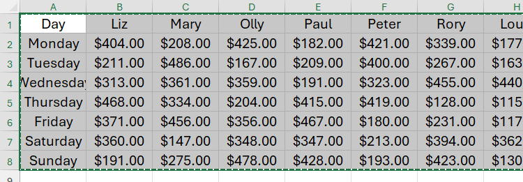
First, select all the data, including the header row, and press Ctrl+C to copy it.
If your data is in a formatted Excel table, before you copy it, you’ll need to select any cell in the table, and click “Convert To Range” in the Table Design tab on the ribbon.
Next, click the cell where you want the top-left value of the transposed data to be (making sure there’s enough space below that cell for the new table), and press Ctrl+Alt+V to launch the Paste Special dialog box.
Once opened, press E to activate the transpose action. Also, double-check whether you want to select any of the options in the Paste section of the dialog box—for example, if some cells are formatted as dates, press U to keep the values and their number formats.
When you press Enter, the transposed table appears in the position you selected.
You can now delete the original table, and format the new one to suit your needs.
You can also use the TRANSPOSE function in Excel to achieve a similar outcome. However, where data transposed through Paste Special isn’t linked to the original data, the TRANSPOSE function produces a spilled dynamic array that updates to reflect any changes in the original data.
Although the Paste Special dialog box lets you copy formats, there’s a quicker way to achieve this if you want to copy formatting to lots of cells in different regions of your spreadsheet. Select the cells containing the formatting you want to copy, and double-click the Format Painter icon. Then, select the cells where you want the formatting to be pasted.
