Here at How-To Geek, we often talk about the benefits of using keyboard shortcuts to speed up your workflow. However, when you’re creating a spreadsheet in Microsoft Excel, the double-click shortcut can be just as useful. In this guide, I’ll share 11 of my favorite double-click Excel tricks.
1
Duplicate a Formula
After typing a formula into a cell and pressing Enter, you might be tempted to click and drag the cell’s fill handle to copy it down a column. However, this can take far too long if your spreadsheet has hundreds or thousands of rows.
Instead, select the cell containing the formula, and double-click the fill handle rather than dragging it.

In an instant, Excel duplicates the formula down the column until it reaches a blank row. This is one of the reasons why it’s generally considered good practice to avoid having blank rows in an Excel dataset.

If your data is formatted as an Excel table, the column will automatically populate after you type the first formula and press Enter.
2
Enter Cell Edit Mode
In the example above, the result in cell D5 returned an error because it’s not possible to divide a number by zero. One way to fix this is to re-enter the cells and edit the formula.
Related
How to Fix Common Formula Errors in Microsoft Excel
Find out what that error means and how to fix it.
Cells in Microsoft Excel have four modes—ready mode (the default state), enter mode (activated when you start typing something into a cell), point mode (which lets you select cell references using your mouse when typing a formula), and edit mode (when you need to change a cell’s content)—and it’s the latter of these that we need to activate to change the formulas.
To enter a cell’s edit mode, simply double-click it—you don’t need to clear the cell and type its contents from scratch! If a cell contains a formula, the precedent cells become highlighted in different colors.

At this point, you could double-click one of the references in the formula, then single-click another cell to change that reference. However, in this case, we need to embed the existing formula within the IFERROR function.

Related
Then, after you press Enter, double-click the fill handle to reapply the new formula to the other cells in the column.

3
Show and Hide the Ribbon
Because Microsoft Excel has so many tools, the ribbon takes up a large amount of real estate. This can make working in the program difficult if you have a small screen or a large spreadsheet.
Fortunately, you can increase your spreadsheet’s screen space by double-clicking any tab to hide the ribbon.
Now that the ribbon is hidden, notice how much extra screen space you have to work on your spreadsheet.

To reopen the ribbon, double-click any tab again.
4
Rename a Worksheet
If you have more than one active worksheet tab in your workbook, renaming them helps to clarify what each sheet contains, improves your workbook’s accessibility, and improves 3D referencing efficiency.
The quickest route to renaming a worksheet is to double-click its corresponding tab at the bottom of the Excel window, type the new name, and press Enter.

5
Resize Columns
In Excel, columns that are too narrow can cut off important data, and columns that are too wide can unnecessarily take up extra space.
In this example, column A is too narrow, and columns B to D are too wide.

Double-clicking the right edge of a column header resizes the column width to the largest value in that column.

What’s more, you can repeat this action after selecting several columns to avoid having to automatically resize columns one by one.

To do this to every active column in your spreadsheet, single-click the “Select All” button in the top-left corner of the Excel window, and then double-click one of the boundaries between any two column headers.

You can also use the same trick to automatically resize the height of a row—simply double-click the boundary between two row headers to see the row above resize to the tallest element it contains.
6
Copy Formatting Repeatedly
Excel’s Format Painter tool is an invaluable time-saver, as it lets you duplicate formatting from one cell or object to another. However, if you need to duplicate that formatting to more than one element, clicking the Format Painter button each time takes too long.
Instead, you can double-click the Format Painter button to keep the tool active as you apply the formatting to any cell or object you subsequently click.
In this example, let’s say you want the males in blue and the females in green, as is already the case in cells A2 and A3.

To do this, select the cell containing the formatting you want to copy, and double-click the “Format Painter” icon in the Home tab on the ribbon.

Then, after seeing the cursor change to a paintbrush symbol, click each cell to which you want to apply the formatting. Then, click the Format Painter icon again (or press Esc) once you’re done.

Format Painter also applies to shapes, tables, and charts, and it even copies conditional formatting rules.
7
Jump to the Edge of a Range
Scrolling up, down, left, and right on a large worksheet can be frustrating and time-consuming, especially if you want to jump to the far edge of your data.
To save time, double-click one of the four edges of a cell to jump to the edge of the range in that direction.
In this example, double-clicking the top edge of cell C7 would activate cell C1, double-clicking the right edge would take me to cell D7, double-clicking the left edge would jump to cell A7, and double-clicking the bottom edge would activate cell C27, the lower edge of the range.

The cell you double-click doesn’t have to be at the edge of the range—you can jump to an edge from wherever you are in the range.
Hold shift as you double-click the edge of a cell to select all the cells between the active cell and the outer cell, inclusive.
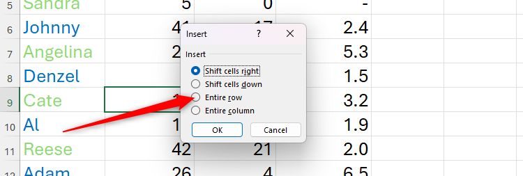
In Excel’s dialog boxes, you can double-click a tool to avoid having to also click “OK.”
This double-click trick doesn’t work with checkboxes in dialog boxes. Clicking these twice selects and deselects the corresponding option.
Here, after right-clicking a cell and selecting “Insert,” I can double-click the words “Entire Row” or the radio button to activate that option and close the dialog box.
In a second example, after selecting column A and row 1 and pressing Ctrl+1, I can double-click “Text” in the Number tab to change the number formats and close the dialog box.


Related
Excel’s 12 Number Format Options and How They Affect Your Data
Adjust your cells’ number formats to match their data type.
9
Activate a Chart’s Format Pane
After creating a chart in Excel by selecting some data and clicking one of the options in the Insert tab on the ribbon, you can double-click any of the chart’s elements to launch the corresponding Format pane.

Related
Then, with the Format pane still open, you can single-click any other part of the chart to format that element.

10
Change a PivotTable’s Field Settings
One of the most common challenges I see people face when using PivotTables in Excel is knowing where to find the right settings to adapt the data for easy analysis.

In this example, the Games Per Goal column is represented as a count, not a sum, so this needs to be changed.
The quickest way to do this is to double-click the center of the field header in the first row of the PivotTable.

Then, in the Value Field Settings, dialog box, double-click the correct aggregation type to select it and close the window.

You can also double-click the field header to alter the number formatting. For example, to fix the inconsistent decimalization in the example below, you would need to double-click the field header, then single-click Number Format in the Value Field Settings dialog box.

Then, double-click “Number” in the Format Cells dialog box to force all numbers to have two decimal places.

Now, the PivotTable is displaying the correct aggregation, and the decimal places are all the same.
